Several of the adjustment approaches used in this study require a dataset that is highly representative of the U.S. adult population. This dataset essentially serves as a reference for making the survey at hand (e.g., the online opt-in samples) more representative. When selecting a population dataset, researchers typically use a large, federal benchmark dataset such as the American Community Survey (ACS) or Current Population Survey (CPS), as those surveys have high response rates, high population coverage rates and rigorous probability-based sample designs.
One limitation of using a single survey, such as the ACS, is that the only variables that can be used in adjustment are those measured in the ACS. This means that a researcher could adjust on characteristics like age, income and education but not political party affiliation, religious affiliation or voter registration. One solution is to take several benchmark datasets measuring somewhat different variables and combine them to create a synthetic population dataset.25
Questions that the ACS has in common with other benchmark surveys are used to statistically model likely responses to questions that were not asked on the ACS. The subsequent sections detail how the synthetic population dataset was constructed for this study.
Construction of the synthetic population dataset
The synthetic population dataset was constructed in three main steps:
Researchers downloaded public use datasets for nine benchmark surveys and then recoded common variables (e.g., age and education) to be consistent across the surveys. They then rescaled each survey’s weights to sum to the nominal sample size.
Each dataset was then sorted according to each record’s weight, and divided into 20 strata based on the cumulative sum of the survey weights so that each stratum represented 5% of the total population. Next, a sample of 1,000 cases (interviews) was randomly selected from each stratum with replacement and with probability proportional to the case’s weight. This had the effect of “undoing” the weights and producing a 20,000-case dataset for each survey that was representative of the total population.
These 20,000 case datasets were then combined into a single large dataset. Using that combined dataset, researchers produced 25 multiply imputed datasets via the chained equations approach.
After imputation, only the 20,000 cases that originated from the ACS were kept, and all others were discarded. This was done to ensure that the distribution of the main demographic variables precisely matched the ACS distribution, while the imputed variables reflect the distribution that would be expected based on the ACS demographic profile.
Each of these steps is discussed in detail below.
Dataset selection and recoding

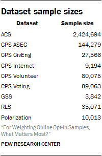
Nine datasets were used to construct the synthetic population dataset: the 2015 ACS, the 2015 CPS Annual Social and Economic Supplement (CPS ASEC), the 2013 CPS Civic Engagement Supplement (CPS CivEng), the 2015 CPS Computer and Internet Use Supplement (CPS Internet), the 2015 CPS Volunteer Supplement (CPS Volunteer), the 2014 CPS Voting and Registration Supplement (CPS Voting), the 2014 General Social Survey (GSS), the 2014 Pew Research Center Religious Landscape Study (RLS) and the 2014 Pew Research Center Political Polarization and Typology Survey (Pol.). Each survey contributed a number of variables to the frame. In all, the frame contains 37 variables, with many of these variables present in multiple surveys.
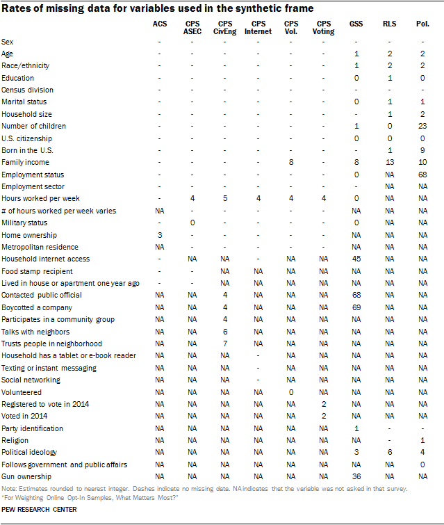
All nine datasets featured a number of common demographic variables such as sex, age, race and Hispanic ethnicity, education, census division, marital status, household size, number of children, U.S. birth, citizenship status and family income. Other variables were only measured in a subset of the surveys. Volunteering, for example, is present only in the CPS Volunteer Supplement, while party identification is only present in the GSS, the RLS and Pew Research Center’s Polarization Survey, none of which are federal government surveys.

Variables that were measured or coded differently across surveys were recoded to be as comparable as possible. This often meant that variables were coarsened. For example, the CPS top-codes age at 85 years or more, so the same coding scheme was applied to all of the other surveys as well. In other cases, this involved treating inconsistent values as missing. For instance, both the ACS and the various CPS surveys ask respondents how many hours they usually work per week. However, the CPS surveys also allow respondents to indicate that the number of hours they usually work per week varies, while the ACS does not have this option. In the above table, missing data for hours worked per week across the CPS surveys is not truly missing; rather, it consists of people who indicated that their hours vary. However, these data are treated as missing for consistency with the way it is asked in the ACS. Imputed values can be interpreted as predicting how those individuals would have answered if they had been asked the ACS question instead.
Stratified sampling
The benchmark datasets differed in sample design and sample sizes. In order to address these differences, we selected exactly 20,000 observations per dataset before appending them together. Sampling was done with replacement and with probability proportional to the case’s weight. The sample size was selected in order to provide enough data for the adjustment methods used while still being computationally tractable. For the CPS Internet Supplement, the GSS and the Polarization Survey, this guaranteed that observations would be sampled multiple times.
We used the relevant weights for each dataset. The person-level weight was used for the ACS, the person supplement weight for the CPS ASEC and the self-response supplement weight for the CPS Civic Engagement supplement. The CPS Internet Supplement was filtered down to respondents who had a random respondent weight, because the texting and social networking variables were only measured for these respondents. The nonresponse weight was used for the CPS Volunteer Supplement, while the nonresponse weight accounting for both cross-section and panel cases was used for the GSS. Full sample weights were used for the RLS and the Polarization Survey. Finally, for the CPS Voting Supplement, the second-stage weights were adjusted as recommended by Hur and Achen26 to correct for bias resulting from item nonresponse being treated as not having voted. Each of these weights was rescaled to sum to the sample size of each of their respective datasets.
To ensure that the samples contained the correct proportion of cases with both large and small weights, each dataset was sorted according to the weights, and divided into 20 strata, each of which represented 5% of the weighted sample.
Imputation
The nine datasets were then combined into a single dataset, and all missing values were imputed via a “chained equations” approach that iterates through modeling each variable as a function of all the others.27 For example, if age, sex and education were the only variables, a chained equations approach might first impute age based on sex and education, then sex based on age and education, then education based on age and sex, and would repeat this cycle for some number of iterations in order to achieve stability. This entire procedure is also repeated 25 times, independently of one another, to produce multiple synthetic frames that can be compared against one another to assess variance stemming from the imputation process. Each frame went through 10 iterations.
There are a wide variety of models that can be used to impute each individual variable dependent on all the others, such as regression models or “hot-deck” methods where each missing value is replaced by an observed response from a “similar” unit. For the synthetic population dataset, each variable was imputed using a random forest “hot-deck” method.28
After imputation, the final synthetic population dataset was created by deleting all but the cases that were originally from the ACS. This ensures that the demographic distribution closely matches that of the original ACS, while the imputed variables reflect the joint distribution that would be expected based on the variables that each dataset had in common.
Evaluating the imputation quality
We took several steps to ensure that the imputation procedure produced results that accurately reflected the original datasets. First, we crossed each of the imputed variables (e.g., voter registration and party identification) with the fully observed variables (e.g., age, sex and education), and for each cell, compared the size of the cell in the ACS dataset to its size in the original dataset from which it was imputed. Overall, the imputed distributions were quite close to the originals. The average absolute difference between the imputed and original values for each cross-classification was 2 percentage points. This means that on average, the imputed values not only matched the distribution for the full population, but also matched the distribution within demographic subgroups.
Although the multiple imputation procedure created 25 versions of the synthetic population dataset, only one of them was used to perform the adjustments in this study. One concern with this approach is the possibility that the results could vary widely depending on which of the 25 synthetic populations was used. Although it was not computationally feasible to repeat the entire analysis on each of the imputed datasets, we did repeat one of the adjustment procedures across all 25 datasets in order to assess the degree to which the imputation procedure may be affecting the study’s findings.
For each of the 25 imputed datasets, we performed raking with both the demographic and political variables on 1,000 bootstrap samples of n=3,500 following the same procedure that was used in the body of this report. For each substantive category in the 24 benchmark variables, we calculated the weighted percentage for each bootstrapped sample. Then we calculated the total variance (mean squared error) for each estimate with all 25,000 bootstrap samples combined. Finally, we calculated the variance for each of the 25 sets of estimates separately and took the average. This is the within-imputation variance. This process was repeated for all three vendors.
If the total variance is much larger than the within-imputation variance, then estimated variability and margins of error that use only a single imputation (as was done in this study) would be underestimated. In this case, the total variance was only 1.002 times as large as the average within-imputation variance. This means that the estimated variability described in the report is for all practical purposes the same as if the analysis had been repeated for all 25 imputations.
The reason the two are so close is likely due to the fact the imputation only affects the variability of the survey estimates indirectly, and makes up only a small portion of the survey variability. If we were to compare the total and within-imputation variability for the imputed values themselves (as we might if the synthetic population dataset were the main focus of the analysis rather than simply an input to the weighting), the difference would likely be larger.
Adjustment variables used in the study
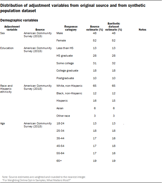
The core demographic adjustment variables used in the study were 6-category age, sex, 5-category educational attainment, race and Hispanic ethnicity, and census division. The expanded political variables add to this 3-category political party affiliation, 3-category political ideology, voter registration, and whether the respondent identifies as an evangelical Christian.
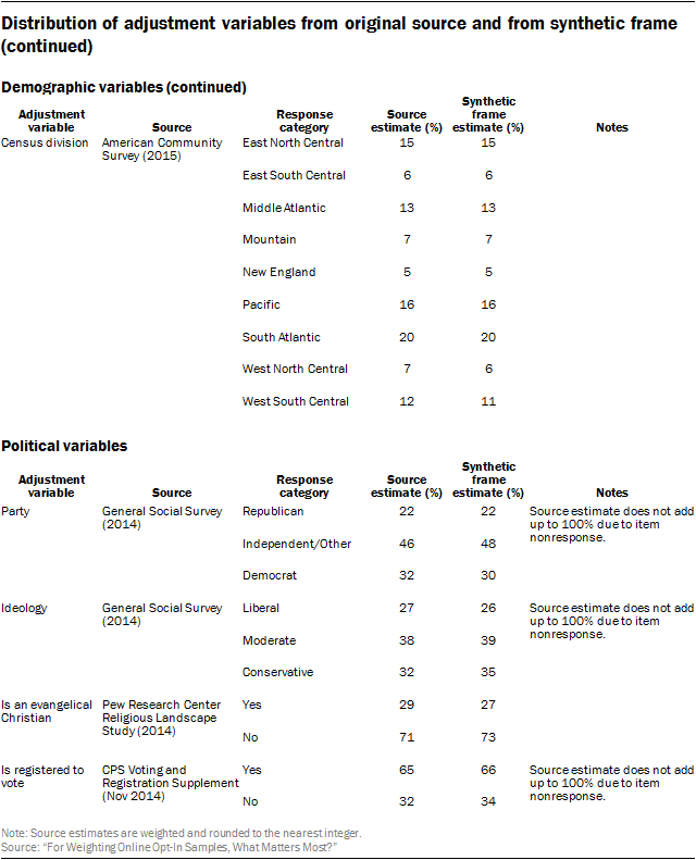
The following table compares the distribution of the adjustment variables on the synthetic population dataset versus from one of the original high-quality survey datasets used to create the synthetic dataset. All demographic variables were fully observed on the ACS, so the synthetic frame will differ from the original source only on the set of expanded political variables.
The largest difference between the source survey and the synthetic frame was on political ideology. The estimated share of self-described conservatives was 32% in the GSS versus 35% in the synthetic frame. The latter estimate is similar to measures from Pew Research Center’s Religious Landscape Study and the Political Polarization and Typology Survey, which were also used in the frame. The exact reason for this discrepancy is unclear, but there are several potential factors. Unlike the Center’s measures, which are collected via live telephone interviewing, the GSS question is administered in-person using a showcard. In addition, the GSS question uses a seven-point scale, while the Center’s questions use a five-point scale. Finally, there may be important differences between the demographic makeup of respondents to the GSS and respondents to the ACS.


