In a recent study about online opt-in polling, Pew Research Center compared a variety of weighting approaches and found that complex statistical adjustments using machine learning don’t perform much better than raking, a simple weighting technique that pollsters have used for decades. Instead, accuracy depended much more on the choice of variables used in the adjustment. We were able to achieve greater accuracy using an expanded set of politically-related variables than we were using demographics alone.
Since then, a number of people have asked us why we didn’t include multilevel regression and poststratification (MRP) in our study. MRP is an increasingly popular approach to survey estimation because it lets researchers perform complex adjustments with many variables and complex interactions without increasing the margin of error as much as would occur using more conventional methods. This makes it particularly appealing for online opt-in surveys, which may require extensive adjustment.
Our main reason for not using MRP in our recent analysis was practicality. MRP requires a separate model for every single outcome. If you have a survey with 40 questions, you would need to run MRP 40 times. By contrast, the methods we looked at (raking, propensity weighting and matching) all assign a single weight to each case in the sample. The procedure only needs to be run once, and the resulting weight can be used to perform a wide variety of analyses on any number of variables in the survey.
Nevertheless, the extra work required for MRP might be worth it if it provided more accurate survey estimates. To see if this is the case, we looked at MRP using data from the three opt-in samples that we collected for our report. The data can be found here. Each sample came from a different vendor but was administered through a common questionnaire.
Due to the difficulty of fitting separate models for each of the 24 benchmark outcomes used in our report, we instead focused on the four benchmarks that showed the largest biases prior to any weighting. These were: voting in the 2014 midterm election, having volunteered in the past 12 months, voting in the 2012 presidential election, and personal tablet use. We also limited our comparison to only adjustments using a simulated sample size of 2,000 and the expanded set of adjustment variables that included both core demographics (age, sex, educational attainment, race and Hispanic ethnicity, and census division) and variables associated with political attitudes and behaviors (party identification, ideology, voter registration and identification as an evangelical Christian). For simplicity, we’ll only show the results for one of the three opt-in samples from our report, but all of the samples yielded similar results.
How does MRP work?
As the name suggests, MRP can be divided into two steps. The first step is multilevel regression. This involves fitting a regression model to survey data where the outcome of interest is the dependent variable and adjustment variables are the predictors. We included main effects and all two-way interactions for the demographic predictors and main effects for the political variables. Each term in the regression model receives a varying intercept, also known as a “random effect.” We fit our model using a fully Bayesian approach with the R package brms, which relies on the Bayesian modeling language Stan.
Below is an example showing how this looks in R. Here, we fit a model predicting whether someone voted in the 2014 general election (VOTE14):
library(brms)
fit <- brm(formula = VOTE14 ~ 1 + (1 | GENDER) + (1 | AGECAT4) + (1 | EDUCCAT5)
           + (1 | RACETHN) + (1 | DIVISION) + (1 | PARTYSCALE3) + (1 | IDEO3)
           + (1 | EVANGELICAL) + (1 | REGISTERED) + (1 | AGECAT4:EDUCCAT4)
           + (1 | AGECAT4:WHITE) + (1 | AGECAT4:GENDER) + (1 | AGECAT4:REGION)
           + (1 | EDUCCAT4:WHITE) + (1 | EDUCCAT4:GENDER) + (1 | EDUCCAT4:REGION)
           + (1 | WHITE:GENDER) + (1 | WHITE:REGION) + (1 | GENDER:REGION),
           # The outcome in our data is binary, so we do a logistic regression.
           data = df, family = bernoulli(link = "logit"),
           # Bayesian models require prior distributions for the parameters in the model.
           # brm has default priors, but you can set them yourself too.
           # Some prior choice recommendations can be found here:
           # https://github.com/stan-dev/stan/wiki/Prior-Choice-Recommendations
           prior = c(set_prior("normal(0, 10)", class = "Intercept"),
                     set_prior("student_t(3, 0, 5)", class = "sd")),
           iter = 1000, chains = 4, cores = 4,
           # These options help mitigate potential problems with the model algorithm
           # See http://mc-stan.org/misc/warnings.html for more details
           control = list(adapt_delta = 0.99999,
                          max_treedepth = 15),
           seed = 20180718,
           refresh = 1)
The second step is poststratification. Here you need to know how many people there are in the population for every combination of variables in the regression model. In this case, we needed to know how many people there were for every combination of age, sex, education, race and Hispanic ethnicity, census division, voter registration status, party identification, political ideology, and identification as an evangelical Christian . Because there is no official data source that contains all of these variables for the U.S. population, we generated estimates for the relative size of all of these groups using a synthetic population dataset that combined information from a variety of different surveys. You can read more about that here.
Next, we used the regression model to predict the mean value for each of these groups. For example, we used the model to calculate the probability of voting in 2014 for white Republican men ages 30 to 49 with a high school education or less who live in the West South Central census division, are ideologically moderate, do not identify as an evangelical Christian, and are registered to vote. We repeated this for every possible combination of these variables that exists in the population.
Finally, to get the overall population mean, we took the weighted average across all of these groups, where each group was weighted according to its share of the population. We repeated this procedure for each of the four outcomes.
How does MRP compare to other adjustment approaches?
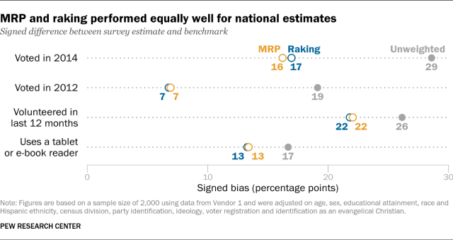
The graph below compares the estimated bias on these four national benchmarks for raking and MRP, using the same set of demographic and political variables, as well as the unweighted data. For national estimates, MRP and raking performed equally well in terms of bias reduction. On its own, this would suggest that MRP does not offer any advantages over raking when it comes to national estimates. As we demonstrated in our report, finding better adjustment variables would have a larger impact on bias reduction.
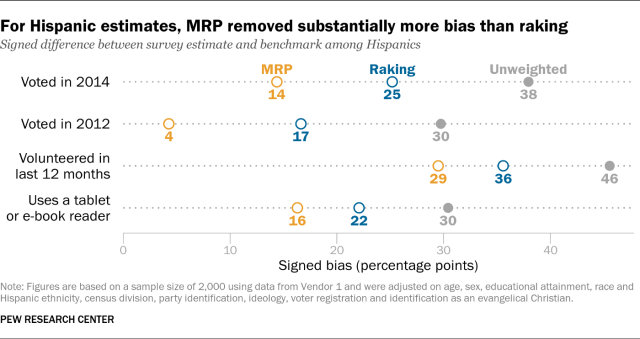
On other subgroup estimates, the results of the MRP-versus-raking comparison were mixed. Raking yielded more accurate estimates for whites and adults with a high school education or less. MRP yielded more accurate estimates for college graduates.
Why did MRP do so much better for Hispanics in particular? One of the adjustment variables we used was voter registration, which is highly correlated with turnout. In the sample from Vendor 1, registered voters overall were overrepresented by 17 percentage points before weighting. But among Hispanics, registered voters were overrepresented by 36 percentage points. In our report, we weighted on registration status for the sample as a whole, but not within subgroups. Even after weighting, the share of Hispanics who are also registered to vote was still 14 percentage points too high. By contrast, in the MRP model, the poststratification step automatically ensured that the share of registered Hispanics matched the population.
As it turns out, if you weight voter registration within race/ethnicity, raking comes much closer to MRP on the share of Hispanics who voted in 2012, but it’s still a few points too high. This suggests that while voter registration is a big part of the story, there are still other differences that aren’t accounted for in the raking.
How precise are MRP estimates?
Of course, bias is only part of the story. One downside of weighting on many variables and their interactions is that it tends to lead to more variable estimates (i.e. a larger margin of sampling error). The main advantage of MRP is that it lets researchers perform these kinds of complex adjustments without the same penalty to precision. But how do MRP and raking compare in terms of variance?
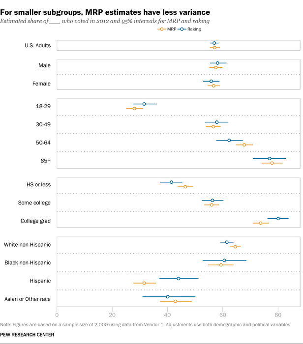
In this case, we found that MRP and raking produced very similar 95% intervals for national estimates of the share who voted in 2012 — both were plus or minus 2 percentage points. However, MRP did produce more stable estimates for smaller subgroups. With MRP, the 95% credibility interval for the estimated percentage of Hispanics who voted in 2012 was roughly plus or minus 4 percentage points, compared to a confidence interval of about plus or minus 7 points with raking. For estimates based on those aged 65 and older, MRP gives an interval that’s again plus or minus 4 percentage points, versus 6 from raking.
Summing up
Our original report found that the most complex adjustment procedure tested performed better than raking at generating estimates for Hispanics. The same can be said for MRP, which has some clear advantages in terms of lower bias and greater precision for some subgroups relative to raking. For analyses focusing on subnational estimates and with just a few outcome variables, MRP makes a great deal of sense. For analyses producing estimates for all U.S. adults (rather than subgroups) on a large number of survey questions, the relative advantage of MRP is less clear and the added computational difficulty appears harder to justify.


